A Research Project in Computational Electrodynamics
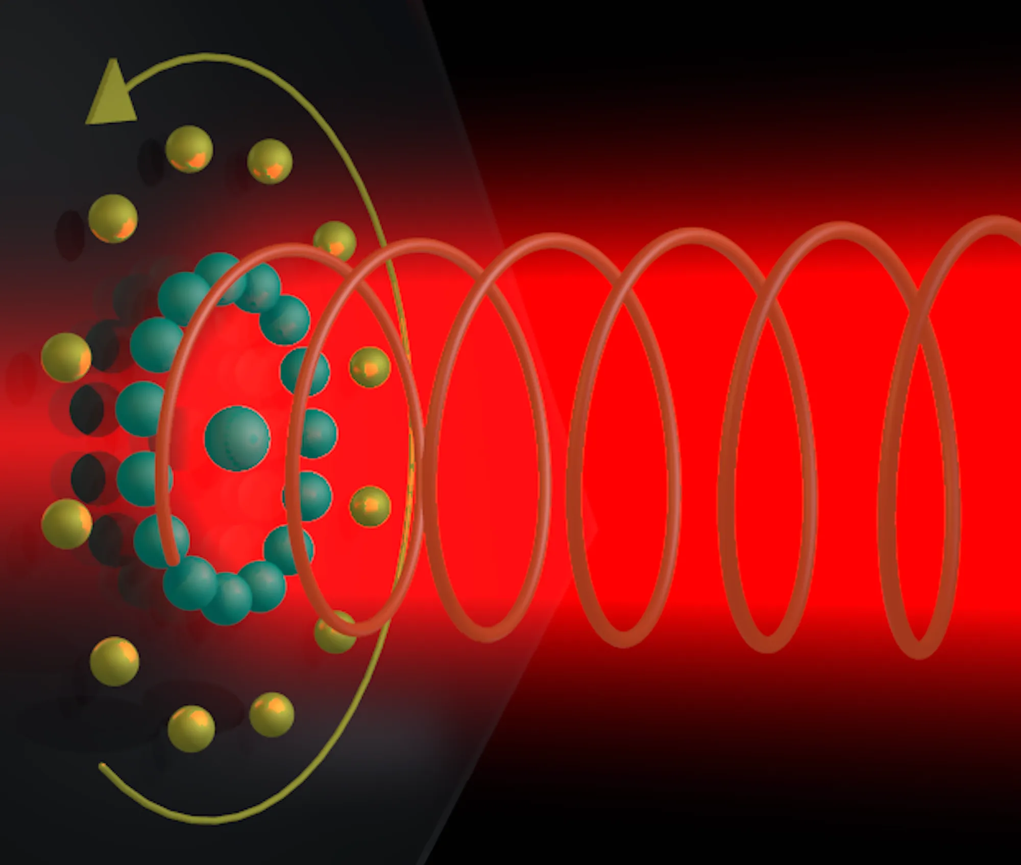
When I was a postdoc I continued my graduate research in computational electrodynamics, studying the physical properties of nanoparticle systems illuminated by light. Nanoparticles in solution can be localized by tightly focused laser beams, called optical tweezers. This localization is due to intensity and phase gradient forces from the trapping laser. When multiple nanoparticles are trapped in a single optical tweezer, they electrodynamically interact with each other through scattered radiation to form structured arrays called optical matter. These optical matter structures exhibit novel physical properties, such as non-conservative and non-reciprocal mechanical forces.
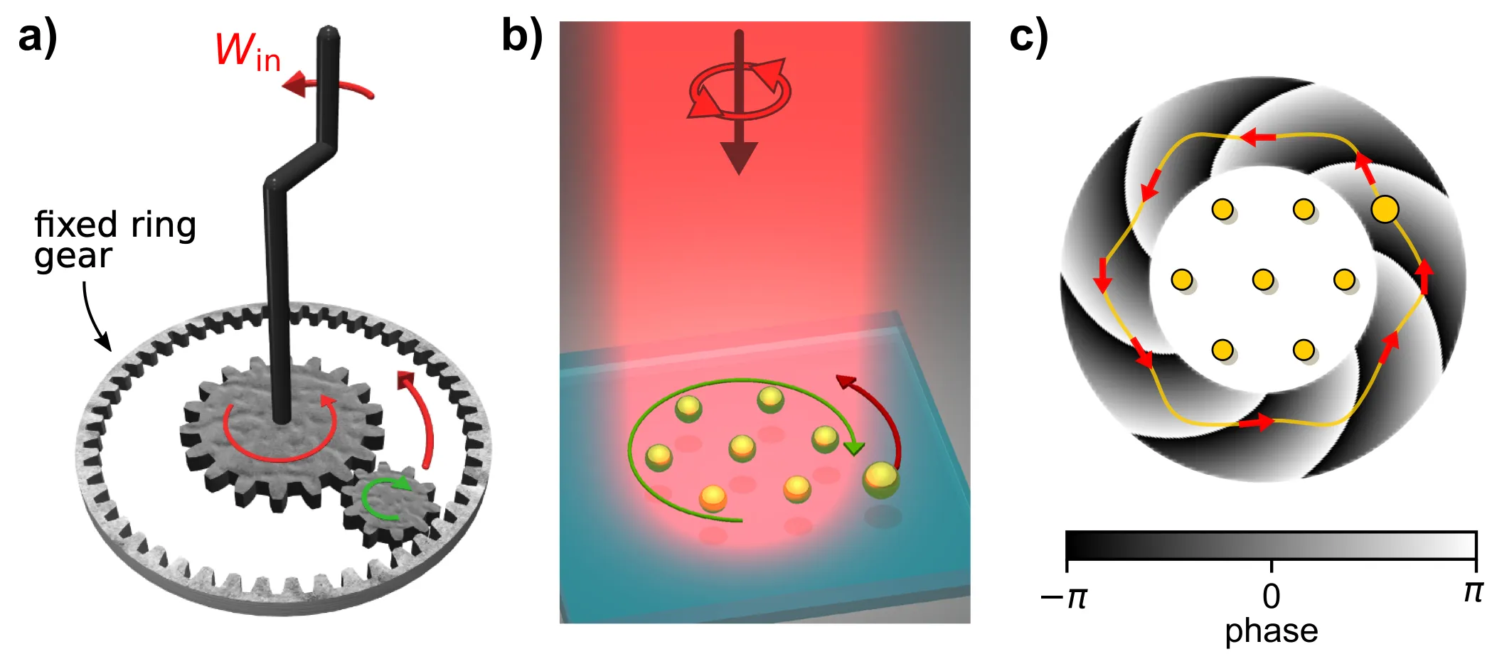
Unfortunately, a lot of my postdoc research ideas were short-lived, as I transitioned to HPC and later Software Engineering in industry. There was one research project in particular that always fascinated me, but I only ever scratched the surface. This work would be a direct extension of my paper on optical matter machines, a demonstration that optically bound nanoparticles can behave like two interlocked gears.
I was hoping to expand this work in the following direction:
- Instead of trapping the central 7 nanoparticles (center gear), those particles could be optically printed onto the substrate at precise positions to form a fixed, immobile array.
- A single probe particle would move in the scattered electrodynamic force field from that central array.
- Because the dynamics only involves a single particle, the Fokker-Planck equation can be solved directly to obtain steady-state probability density and currents of the probe’s position.
- This would enable studying non-conservative forces produced by fixed, patterned arrays that could be engineered to optimize the non-conservative effect.
Alas, since I left academia, there is no time to study such interesting physical systems! Configuring computational experiments, inspecting results, trying various approaches… that’s a full-time job for a life I left behind. But in 2026, with the rise of agentic AI, perhaps I could do computational physics research, with only a fraction of my time. So I decided to try building an autonomous research agent with the ambitious goal of conducting end-to-end research and writing a paper, fully autonomously. My motivation was two-fold: (1) I wanted to study the limits of what agents can do autonomously over many iterations, and (2) my passion for computational physics never left, only my time to pursue it had vanished!
An Autonomous Research Agent
To build an autonomous research agent, we need several ingredients:
- Research Objective: this is the objective of our research, what we know about the system, what is interesting to explore, and the type of output paper we want to work towards.
- Local Environment: the agent will run inside an environment with a filesystem, a Python virtual environment, and necessary dependencies and tools installed (e.g.,
numpy,matplotlib,latexmk). For this problem, the environment also needs physics solvers for Maxwell’s equations and the Fokker-Planck equation. - Tools: the agent needs access to pre-created computational physics tools that it can reuse or adapt as it conducts its research.
- Journal: the agent needs memory. Just like a real scientist, a journal system is the perfect way to write findings and store output data artifacts and plots. This allows future runs of the agent to reflect back on previous findings.
- Agent Harness: a harness sets the course for the agent to operate iteratively. It instructs how to pursue the research goal within the local environment, how to use tools, and when to stop research and wrap-up a journal entry
Research Objective
The research objective is stored in a top-level Markdown file OBJECTIVE.md. Here is a snippet:
A free nanoparticle (the “probe”) moves under optical and electrostatic forces in the vicinity of a fixed array of nanoparticles illuminated by a focused laser beam. Because the illumination is circularly polarized, the optical force field acting on the probe is non-conservative — it cannot be derived from a scalar potential. The goal is to understand the steady-state behavior of the probe particle outside the cluster, where emergent non-conservative dynamics may occur.
The objective also states the research deliverables:
- Journal entries documenting findings at each iteration
- Python scripts or notebooks with reproducible computations and figures
- A publication-quality LaTeX paper (paper/main.tex) — abstract, introduction, methods, results, discussion, references, figures with captions, equations
and the key scientific questions:
- Exterior steady-state trapping: Does the probe localize in an annular region outside the cluster? What is the shape of the steady-state probability distribution in this exterior region?
- Non-conservative circulation: Does the non-conservative optical force field produce persistent probability currents (circulation) around the exterior of the array? What are the angular velocities and circulation patterns?
- Balance of forces: How does the interplay between electrostatic repulsion (preventing contact), optical binding (providing attraction at ~λ/n), and non-conservative curl (driving circulation) create the exterior steady state?
- Tunability: How do surface charge, Debye length, beam parameters, and array geometry control the exterior circulation? Can we optimize for maximum circulation rate or specific trapping patterns?
- Emergent dynamics: Are there qualitative transitions (e.g., from localized trapping to free circulation, hopping between binding sites, bistability) as parameters are varied?
Local Environment
The local environment is a Python virtual environment managed by uv.
Installed into the virtual environment:
- MiePy: my computational electrodynamics solver. It solves Maxwell’s equations for particles illuminated by arbitrary beams.
- FPlanck: my Fokker-Planck solver. It solves for the steady-state probability distribution of particles in arbitrary force fields.
- StokeD: my Stokesian dynamics solver. It solves particle trajectories for particles in solution with hydrodynamic interactions.
With these three tools, a researcher (and an agent!) can study the fascinating dynamics of optical matter systems. The environment has additional tools for data analysis, file IO, and LaTeX documentation.
Computational Physics Tools
Predefined scripts act as tools that the research agent can invoke at any point during its work. These scripts serve as “building blocks” for research:
| File | Purpose | Input | Output |
|---|---|---|---|
force.py | Optical force on a pair of spheres via miepy T-matrix | Two particle specs (radius, material, position), wavelength, beam config | Force vectors (pN) on each particle + separation |
force_field.py | 2D optical + DLVO force map for a probe scanned over a grid near fixed particles | Fixed particle array, probe spec, 2D grid bounds, beam config, DLVO params | HDF5 with force_field[3, Nx, Ny], grid axes, force stats |
fokker_planck.py | Steady-state probability distribution from a precomputed force field via fplanck | Path to force field HDF5, temperature, boundary condition, barrier height | HDF5 with steady_state[Nx, Ny], probability current, curl |
langevin.py | Brownian dynamics trajectory of a probe particle (miepy forces computed on the fly via stoked) | Fixed particles, probe spec + start position, beam config, timestep, n_steps | HDF5 with positions_nm[n_steps, 2], time, MSD |
scattering.py | Cross-section spectra + multipolar decomposition over a wavelength range | Particle cluster, wavelength list, beam config, lmax | HDF5 with scattering/absorption/extinction arrays, per-multipole breakdown |
The research agent is also at liberty to use these tools as a reference to build new tools when writing Python scripts in its journal.
Journal System
Scientific journalling is done in the filesystem at the top-level journal/ folder.
journal/INDEX.md tracks one line per entry that summarizes the outcome of that entry succinctly.
Each entry is a subfolder, e.g., 01-baseline-force-field is the first entry.
The agent can create any files here, mostly Python scripts.
Output artifacts such as png and h5 files are written to an artifacts/ subfolder.
The final action of the agent is to write a FINDINGS.md file, which contains specific details about this entry beyond what was written in INDEX.md.
An example of the journal/ filesystem with a single research entry:
- INDEX.md
- 01-baseline-force-field
- artifacts
- angular_analysis.png
- circulation_analysis.png
- force_analysis.png
- force_field_coarse.h5
- force_field_fine.h5
- force_field_xpol.h5
- fp_coarse.h5
- fp_fine.h5
- fp_xpol.h5
- langevin_trajectories.png
- orbital_analysis.png
- overview_coarse.png
- rhc_vs_xpol.png
- streamlines.png
- traj_rhc.h5
- traj_xpol.h5
- analyze.py
- circulation.py
- compute_fields.py
- FINDINGS.md
- langevin_sim.py
- orbital_estimate.py
- visualize.py
Agent Harness
The agent harness is managed by using the Claude Agent SDK running Opus 4.6.
Launching the agent for research iterations is done simply invoking a top-level main.py file:
uv run main.py -n 5Each research iteration has a fresh context window, and loads context like so:
- Reads
OBJECTIVE.mdto understand the research objective. - Reviews
journal/INDEX.mdto see a short summary of all previous iterations. - Receives a system prompt that instructs how to use tools within the Python environment to work towards the objective, and encourages building on previous entries or researching the unexplored.
- Is encouraged to investigate
journal/<ENTRY>/FINDINGS.mdfor further details on past iterations. This is similar to progressive disclosure in agent skills, where detailed context is only loaded as needed.
Below are examples of the single-line journal/INDEX.md lines for the first five research iterations.
01-baseline-force-field
CPL produces non-conservative circulation (10 kT/orbit at binding distances, Pe~10) around 7-Au hexagonal array; 100% exterior confinement with DLVO; x-pol gives exactly zero circulation
02-power-dependence
Circulation scales exactly linearly with power (0.92 pN·nm/mW); Pe=1 threshold at ~9 mW; sharp exterior→interior confinement transition at ~142 mW when optical force overcomes DLVO in interstitial gaps
03-wavelength-dependence
Circulation peaks at cluster LSPR (680 nm) with 9.1× enhancement over 800 nm baseline; but resonance destabilizes confinement (radiation pressure expels probe); optimal spectral window at 720–760 nm balances circulation (2.4–5.7× enhancement) with exterior confinement
04-spacing-dependence
Optimal spacing d≈λ/n=600 nm maximizes near-field circulation (2088 pN·nm, 2.7× baseline); cluster resonance self-tunes to optimal spectral window; binding-radius Pe plateaus at ~12–13 for d≥600 nm; sharp confinement loss at d≈750–800 nm
05-array-geometry
Center particle is critical: hex ring alone (N=6) traps probe at center (0% exterior), adding center particle gives 100% exterior confinement; circulation scales ~linearly with N (~120 pN·nm/particle); N=19 two-shell traps between shells (18% exterior); cluster resonance red-shifts with N
Trial One: 5 Research Iterations
After setting everything up, I ran the research agent for 5 iterations. This produced many figures exploring the 7 nanoparticle hex array as a fixed gear. Unfortunately, all of the results were uninteresting.
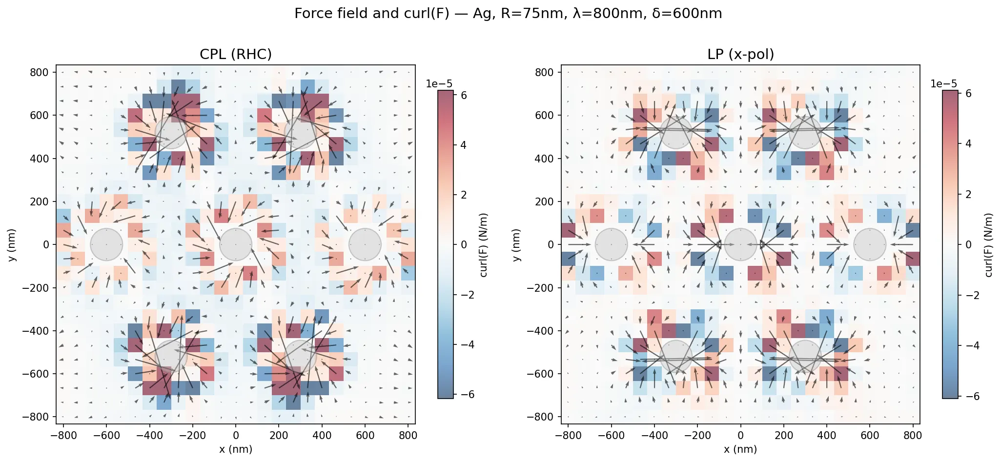
Iteration 1 - Force Field Maps
In the first research iteration, the agent explored the force fields in close proximity of the 7 nanoparticles for circularly and linearly polarized light. The region we actually care about is further beyond what the agent studied (about 1 wavelength, or , beyond the outer particles).
For circularly polarized light, you can see the vorticity in the force field surrounding each particle.
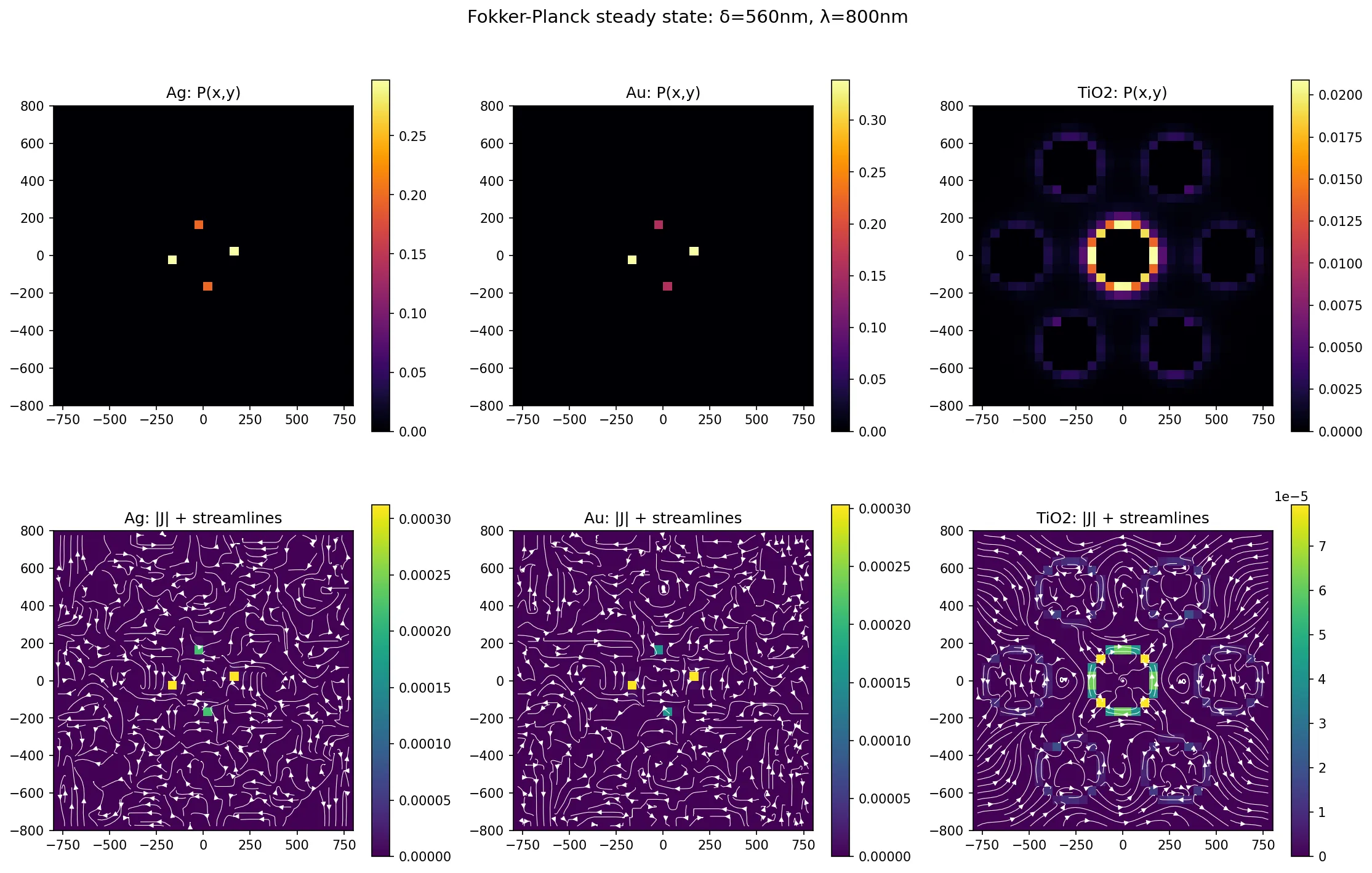
Iteration 4 - Fokker Planck Solution with Different Materials
In the fourth research iteration, the agent solved the Fokker-Planck equation in the near-field of the hex array. The results are that probability is maximized in the near-field of the inner particle. That means a probe particle will simply attach itself to the inner particle. While circulation can be achieved in simulation, in a real experiment this would result in the nanoparticles being chemically bonded as one.
Iteration 5 - Failure
The agent was so impressed with its results in the first five iterations, it suggested the next step was to write a paper:
Suggested next steps (from FINDINGS.md):
- Power dependence — find the critical power below which circulation becomes undetectable
- Linear polarization control — verify circulation vanishes
- Trajectory topology — analyze inter-site hopping patterns
- Begin paper draft — entries 01-05 provide sufficient material
In reality it failed to explore anything of interest. But in the face of failure, the next thing to do is try again!
Trial Two: 34 Research Iterations
After the first trial, I realized a key detail that I had forgotten. These nanoparticles do like to bind in the near-field (direct contact), but often carry a surface charge from ligands on the particle. This charge introduces electrostatic double-layer repulsion, preventing two nanoparticles from getting too close to one another despite the electrodynamic attraction.
For trial two, I introduced a new tool:
| File | Purpose | Input | Output |
|---|---|---|---|
electrostatics.py | DLVO double-layer electrostatic repulsion force between probe and fixed particles | Probe position/radius, fixed particle positions/radii, surface potential, Debye length | 2D force vector (Fx, Fy) in Newtons |
and included electrostatics in the other tools during force computation.
The following was added to OBJECTIVE.md to make it clear the probe needs to stay on the outside of the array.
Critical constraint: the probe must remain outside the fixed array, not trapped in the near-field of any fixed particle. Near-field trapping (sub-wavelength contact) produces trivial, expected physics. The interesting regime is at optical binding separations where the probe orbits or circulates around the exterior of the array under the combined influence of non-conservative optical forces, electrostatic repulsion, and thermal fluctuations.
With these additions, the research iterations produced much more interesting results. I ended up running this trial for 34 iterations, as the agent continued to explore interesting avenues. Here are the stats on what the agent produced over all iterations:
| Type | Count |
|---|---|
| Number of Research Iterations | 34 |
.png files (image artifacts) | 165 |
.h5 files (data artifacts) | 447 |
Lines of .md Markdown (journaling) | 6,428 |
.py files (analysis) | 188 |
| Lines of Python | 42,114 |
| Total disk space | 2 GB |
Below I show some of the interesting figures and results produced at various iterations.
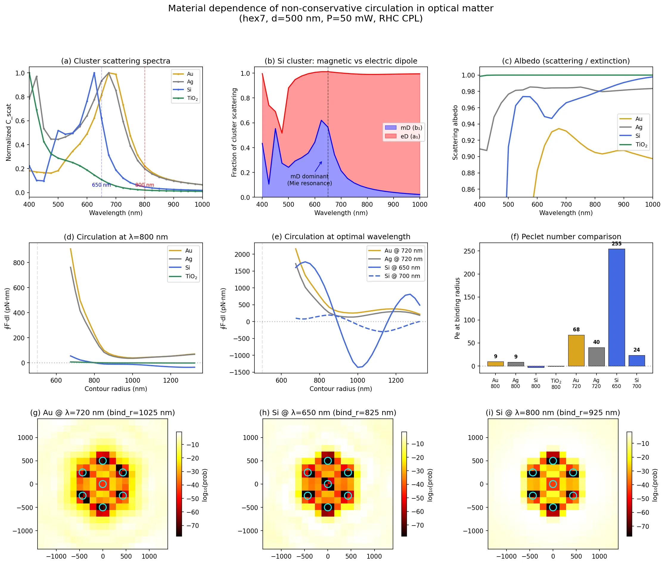
Iteration 7 - Arrays of Different Materials
The agent explored arrays of different materials, noting that Si uniquely has a magnetic dipole resonance.
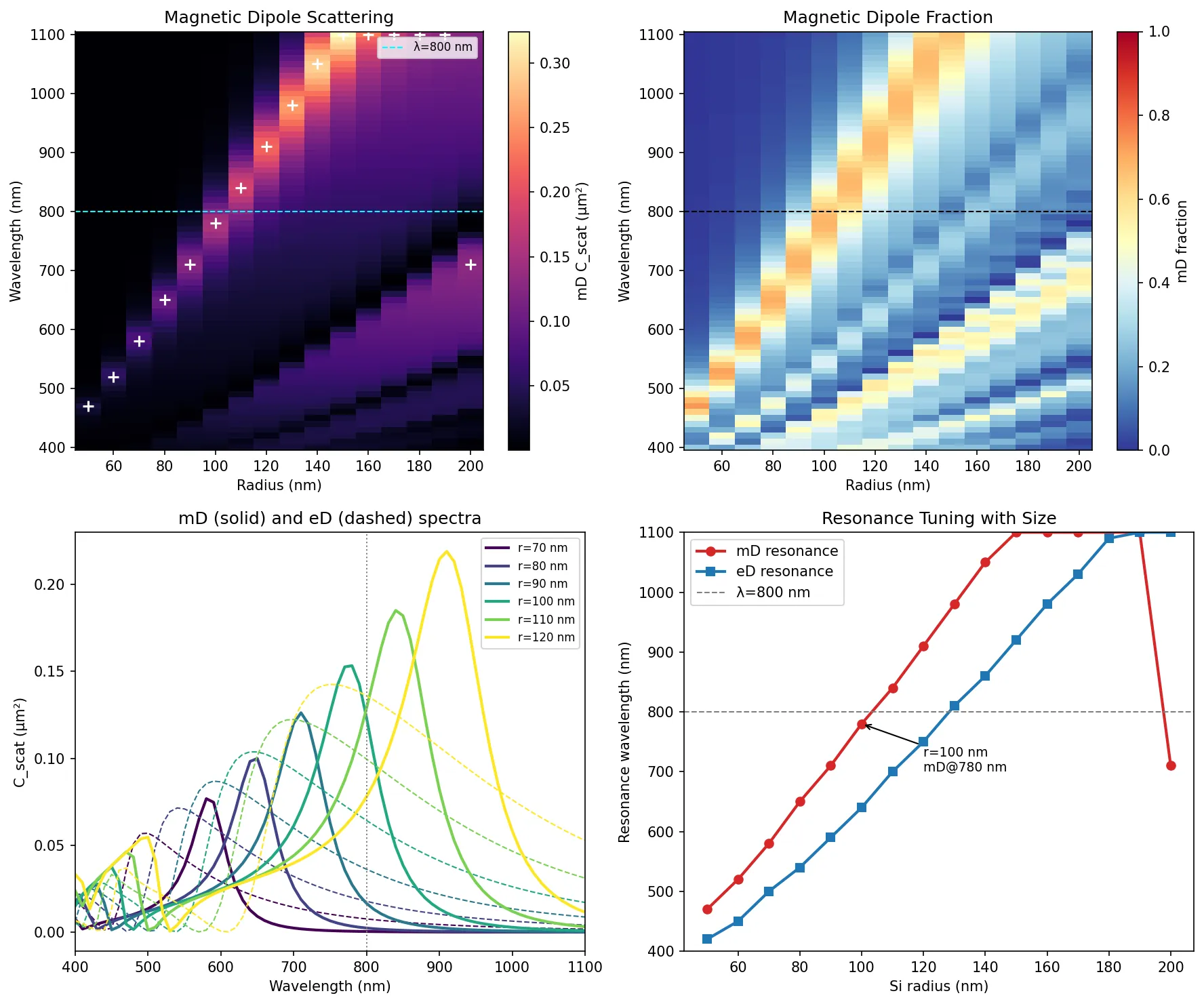
Iteration 8 - Optimizing Magnetic Resonance in Si nanoparticles
The agent optimized the magnetic dipole resonance of Si particles, by finding the optimal particle radius and wavelength window.
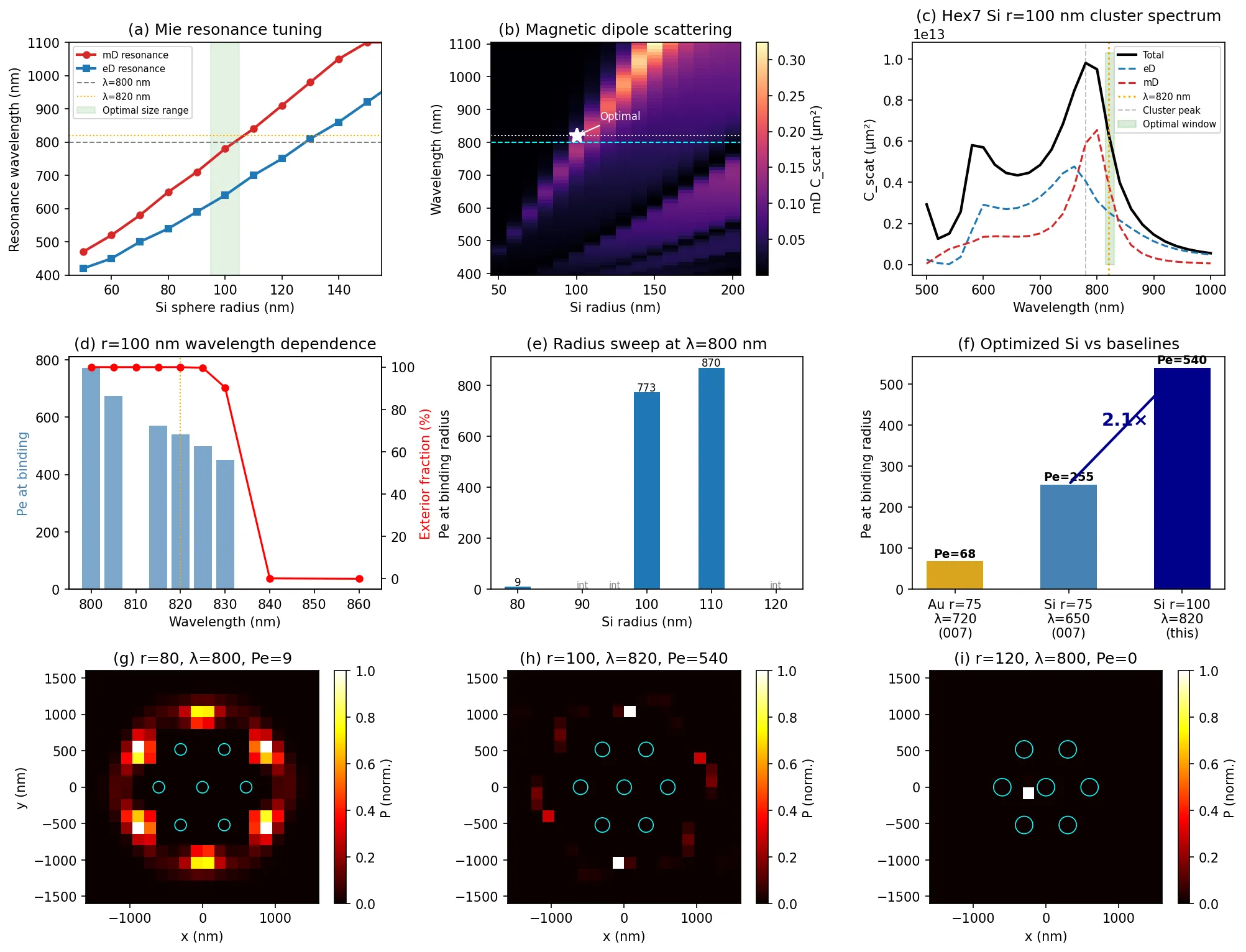
This figure shows in detail how the agent optimized for magnetic dipole scattering:
Iteration 12 - Exploring Array Geometries
In this iteration, the agent explored different geometric configurations of the fixed array. All of these configurations result in subcritical ratchet flows, resulting in the tilted washboard potentials going around the array.
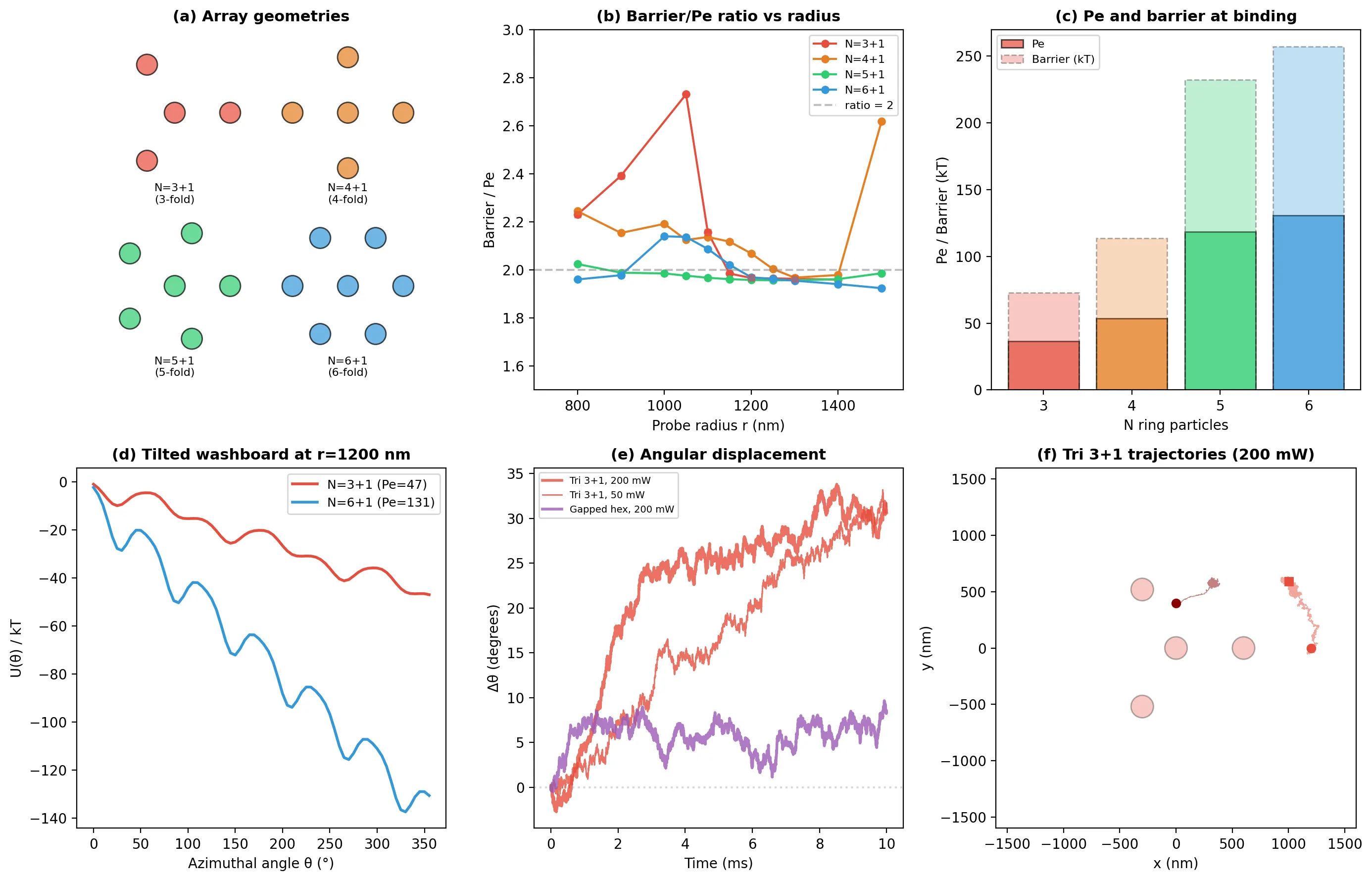
Iteration 14 - Supercritical Flow Achieved
This is the first iteration where the agent created an array that achieved supercritical flow. The ring-like nanoparticle array is effectively converting the incident Gaussian beam into a ring-like potential with circular flow, enabling the probe to flow freely in the confined annulus.
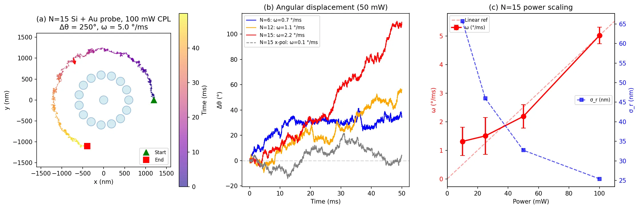
Here is a video of the Langevin dynamics of a single probe circulating in supercritical flow around the ring.
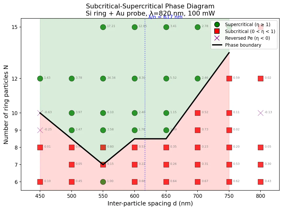
Iteration 19 - Supercritical Flow Phase Space
The agent produced a phase space diagram showing the transition from subcritical to supercritical flow of the probe. At variable spacing of the ring array particles, supercritical flow only happens above some number of particles in the ring .
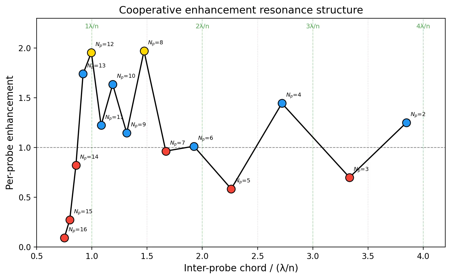
Iteration 24 - Multi-Probe Necklace
Research iteration 24 introduced multiple probes and measured the per-probe cooperative enhancement. Generally, an odd number of probe particles results in weaker flow, whereas an even number (up to ) enhances the flow. At and , the cooperative electrodynamic interactions between the probes result in a 2X velocity increase over the single probe.
Paper Written by Claude
On iteration 26, the research agent wrote a first draft of a paper based on prior results. This paper was refined up through iteration 34 (these later iterations introduced hydrodynamic interactions). Below is the paper: 10 pages, 43 references, 4 figures, 12 equations.
I read the paper in its entirety. Honestly, the autonomous agent did better than I thought it would at this point! The figures could use some work, but I bet this paper could be polished up to make it through peer review at a low-mid tier publisher.
Concluding Thoughts
Claude Opus 4.6 is far more capable as an autonomous research agent in the physical sciences than I thought it would be. This was just an idea I had that I carried through just two trials. I bet with more experimentation and improvements to the tools and harness it could do even better.
Some of my thoughts:
- Experimentation with agents is key. Trial 1 was a failure, but Trial 2 performed much better.
- Trial runs are similar to training ML models - each iteration like an epoch. Expect to run for many epochs to converge, and expect some train runs to get stuck in local minima. If the objective is underspecified, the training will underfit and research in the wrong direction. If it is overspecified, it will overfit and not explore a larger space.
- PhD research isn’t always at the frontier. Often new research is an interpolation between other known research. You’re filling in the gaps, but it’s surrounded by known knowledge. It is these spaces I expect AI agents will have the best capabilities exploring autonomously. Hopefully that leaves humans to perform more work on the frontier.
Shortcomings:
- The paper is OK. There is a more interesting narrative that could be told from the research it did; human guidance is needed to elevate this paper into something publishable (for a first draft it is incredible).
- Generated figures still have many issues in the presentation layer: overlapping elements, poor placement, poor color schemes. These models still need to advance more in vision capabilities within their agentic loop.
- Some avenues were not explored at all, despite being mentioned in the
OBJECTIVE.md. For example, the agent never modified the source beam’s geometry (width or defocus). A human expert is still needed to provide oversight and nudge the research agent in the right direction.