Revisiting code from my grad school days
When I was in grad school, I wrote computational software to perform electrodynamic simulations. The method is known as the Generalized Multiparticle Mie Theory (GMMT), a boundary-condition method for solving Maxwell’s equations for a multiparticle system. In my software implementation, I utilized C++ and OpenMP parallelization for performance-critical code and exposed it to Python via pybind11 for a flexible interface. I used this software package to study the fascinating dynamical properties of nanoparticle systems illuminated by optical tweezers. This software led to many publications and my PhD thesis.
It was during my 6 years in grad school that I discovered my primary passion was writing software, especially high-performance scientific software with powerful, clean user interfaces. I was spending a lot of time writing Python user interfaces, studying modern C++, and distributing my software to collaborators at UChicago, Argonne, and elsewhere. After briefly working in HPC, I transitioned to industry as a Software Engineer, building cloud-based data and compute platforms for a biotech company. As the years went by, I of course left my PhD software behind to collect dust. Despite past collaborators continuing to use my software, emailing me about it, and strangers opening issues on GitHub, I simply had no time to revisit it. Just getting back up to speed would have been a major chore and time-sink.
In 2025, agentic AI upended how software is developed; I experienced this firsthand at my job and quickly pivoted into this new computational paradigm. By late 2025, with Claude Code, Opus 4.6, and all my new software engineering skills, it became apparent that revisiting my grad school software might not be such a hurdle anymore! In just a few prompts, I could be back to developing my grad school software as if I never missed a beat. I allocated some of my spare time to this, largely out of curiosity about agentic AI capabilities in scientific software development, but also to reignite some of the original passion that drove me to grad school in the first place.
Step one was to modernize the software stack. My original code relied on a mess of manual C++ installs and conda packages. Now I know the value of package managers and lock files, so I worked with Claude to do the following:
- Manage C++ dependencies with
vcpkgand CMake - Manage Python dependencies with
uvandscikit-buildbackend - Use
rufflinting & formatting - Configure a GitHub action release pipeline to build wheels for Linux, macOS (ARM), and Windows, and distribute to PyPI
This streamlined development and distribution of the software. Now anyone can run it with one command:
uvx -p 3.13 miepyThis enabled me to address various install issues former collaborators were having.
Then I got curious. Could I revisit some of the ambitious goals I had in grad school for my software, now with the power of Claude Code? So I threw an ambitious problem at Claude: implement a JAX-based GPU backend for the electrodynamic solver to achieve faster solve times at large particle numbers compared to the C++/OpenMP implementation. To achieve this, upfront planning was a must.
Planning with Claude Cowork
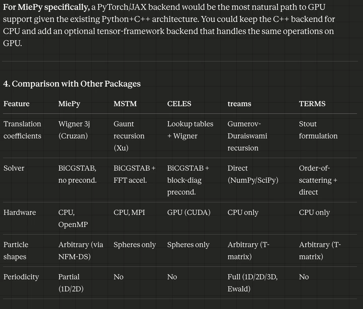
Cowork is a great interface for research that spans a codebase and online literature. In addition to implementing a JAX-based GPU backend, I was asking about general performance improvements we could make. For example, comparing my software to others:
Let’s review the current state of literature relative to how MiePy computes its coefficients to identify potential improvements in performance or algorithm. This could be around (1) how the coefficients are computed, (2) how the matrix system is solved, (3) parallelization or hardware acceleration. We’re looking specifically at this generalized multiparticle mie theory approach
provides a comparison to other solutions available:
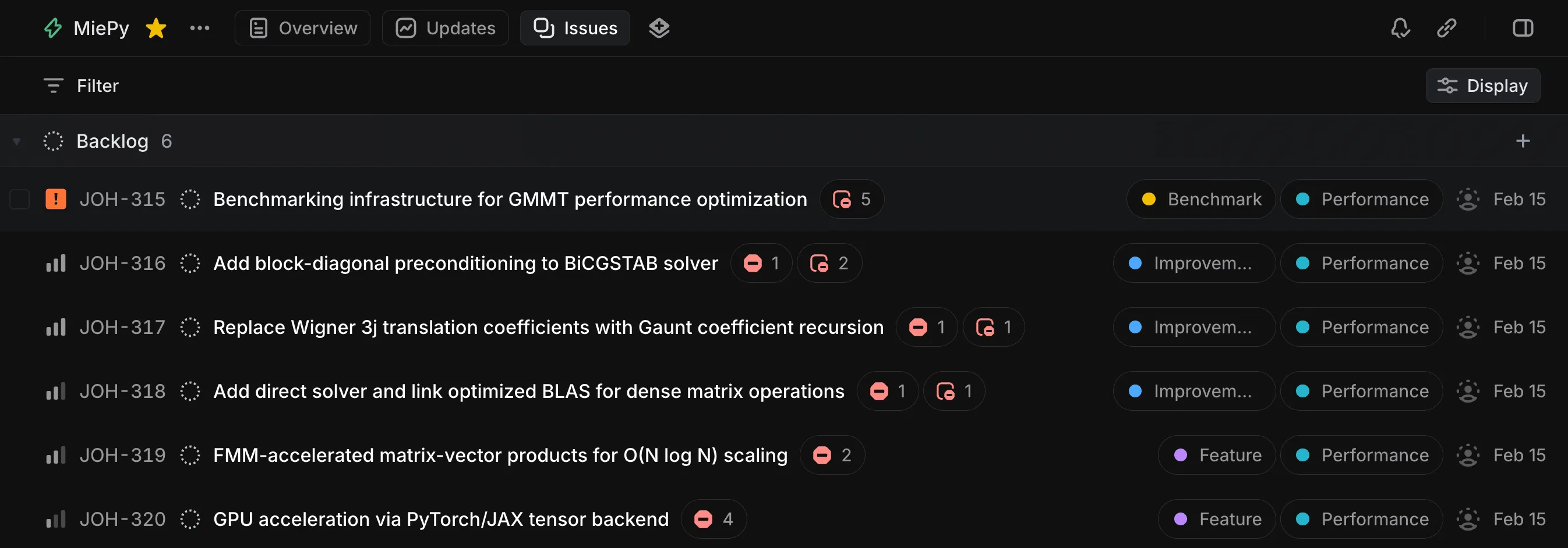
Then I prompted Cowork to help me create a series of Linear issues for improving MiePy’s performance, benchmarking its CPU implementation, and implementing a JAX backend.
There is a linear project named “MiePy”
Let’s create individual issue tasks for these items. Provide plenty of details and external references, including references to existing miepy source code.
In addition to these tasks, there is a preparation task (or tasks) to enable measuring performance. This would enable us to benchmark speed improvement under different conditions. There exist some reference benchmarks already at
src/miepy/examples/benchmarks/but perhaps new ones will be useful, especially for measuring performance at different N particles, or time spent in matrix solver vs building the matrix, or multi-core performance.The goal being, we will start with creating some benchmarks, then start to implement each of these others tasks, measuring benchmarks and running existing test suite for correctness
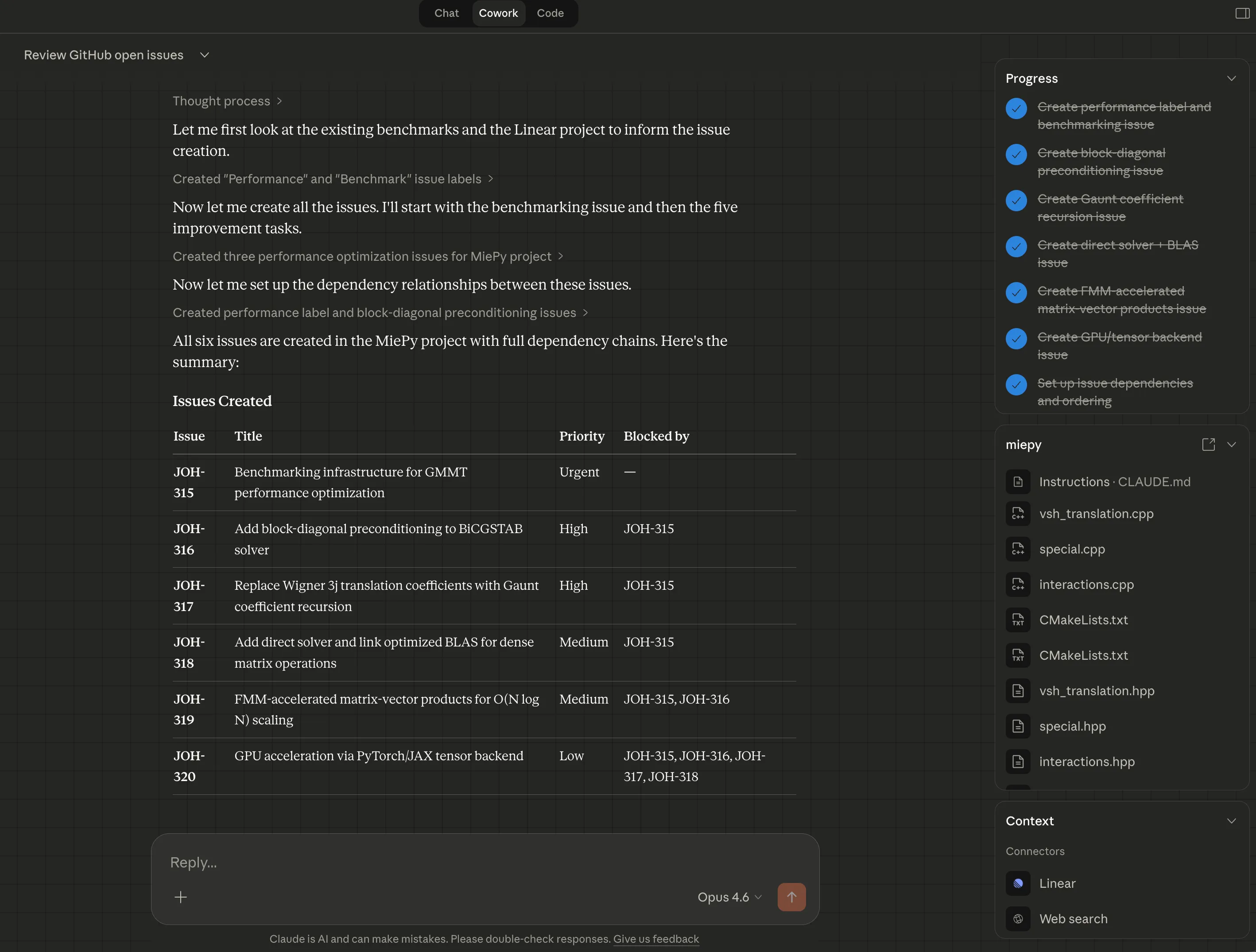
Each Linear issue contains detailed implementation guidance. Additionally, Claude prioritized the issues and established dependencies between them:
The New JAX Backend
There were two parts of the algorithm that Claude ported to JAX:
- Assemble the aggregate T-matrix. Iterate over all particle pairs, compute spherical Hankel functions, Legendre polynomials, Gaunt coefficients, and VSH translation coefficients
- Solve boundary-condition linear system. Use either a direct solver or iterative BiCGSTAB solver to solve the full electrodynamic interactions of the particle system.
These are the only parts of the algorithm that are or (direct solver), with being the number of particles. We might expect a GPU implementation to outperform a CPU one at large .
Implementing #2 was trivial because JAX already provides these solvers:
jax.scipy.sparse.linalg.bicgstab- iterative solverjax.numpy.linalg.solve- direct solver
But implementing #1 is quite non-trivial. The C++ code is highly imperative, and cannot simply be ported and JIT’d. Claude made several notable transformations to accomplish this:
- Split the computation into two phases, where phase 1 runs once to produce XLA constants at compile time.
- Flattened C++ iteration over 4 indices (wave function indices) into a single vectorized dimension
- Padded variable-length Gaunt sums. C++ relied on conditional branching here.
- Converted
complex128intof64real and imaginary components to avoid crippling GPU performance
Here is a snippet from the JAX implementation:
src/miepy/backends/jax/interactions.py
# Step 1: Pair geometry [P = N*(N-1)/2 pairs]
dji = positions[i_vals] - positions[j_vals]         # [P, 3]
rad = jnp.linalg.norm(dji, axis=1)                  # [P]
cos_theta = dji[:, 2] / rad                          # [P]
phi = jnp.arctan2(dji[:, 1], dji[:, 0])             # [P]

# Step 2: Special functions via vmap (Python loops unrolled at trace time)
zn_all = jax.vmap(lambda r: spherical_hn_recursion(p_max, k * r))(rad)  # [P, p_max+1]
Pnm_all = jax.vmap(lambda ct: associated_legendre_recursion(p_max, ct))(cos_theta)  # [P, pnm_size]

# Step 3: Vectorized translation computation
exp_phi = jnp.exp(1j * mu_sum * phi[:, None])         # [P, M]

# A translations: sum_q A_coeff[q] * Pnm[idx_A[q]] * zn[p_A[q]]
Pnm_A = Pnm_all[:, A_pnm_idx]                        # [P, M, Q]
zn_A = zn_all[:, A_zn_idx]                             # [P, M, Q]
sum_A = jnp.sum(A_coeffs * Pnm_A * zn_A * A_mask, axis=-1)  # [P, M]
A_trans = factor * exp_phi * sum_A                      # [P, M]

# B translations: -factor * exp_phi * sum_q B_coeff[q] * Pnm[idx_B[q]] * zn[p_B[q]]
Pnm_B = Pnm_all[:, B_pnm_idx]                        # [P, M, Q]
zn_B = zn_all[:, B_zn_idx]                             # [P, M, Q]
sum_B = jnp.sum(B_coeffs * Pnm_B * zn_B * B_mask, axis=-1)  # [P, M]
B_trans = -factor * exp_phi * sum_B                     # [P, M]

transfer = jnp.stack([A_trans, B_trans], axis=-1)       # [P, M, 2]

# Step 4: Scatter into flat output matrix
# Determine particle index for row/col/mie of each (pair, entry)
row_particle = jnp.where(s_row_is_i, i_vals[:, None], j_vals[:, None])  # [P, E]
col_particle = jnp.where(s_col_is_i, i_vals[:, None], j_vals[:, None])  # [P, E]
mie_particle = jnp.where(s_mie_is_i, i_vals[:, None], j_vals[:, None])  # [P, E]

rows = row_particle * block_size + s_row_local         # [P, E]
cols = col_particle * block_size + s_col_local         # [P, E]

transfer_vals = transfer[:, s_mode_idx, s_ab_parity]   # [P, E]
mie_vals = mie[mie_particle, s_mie_pol, s_mie_order]  # [P, E]
vals = s_sign * transfer_vals * mie_vals                # [P, E]
Verifying correctness
Arriving at the correct solution required setting up the agent to test its results against the existing, working C++ implementation. Agents excel when they can test against an existing reference implementation. The following unit tests verified correctness of individual functions:
| Function | Tests | Reference |
|---|---|---|
| spherical_jn/yn/hn | real z, complex z, derivatives | cpp_special.* |
| spherical_hn_recursion | nmax up to 15 | individual cpp_special.spherical_hn calls |
| riccati_1/2/3 | nmax up to 10 | NumPy/scipy miepy.special_functions |
| associated_legendre | 20 (n,m) combos, including negatives | cpp_special.associated_legendre |
| associated_legendre_recursion | nmax up to 8, all modes | individual C++ calls |
| pi_func/tau_func | general + pole cases (θ=0, θ=π) | cpp_special.* |
| Emn | n up to 8 | cpp_vsh.Emn |
| wigner_3j | known values + selection rules | cpp_special.wigner_3j |
| wigner_3j_batch | 6 parameter combos | individual C++ calls |
| gaunt_batch | 10 (m,n,u,v) combos | cpp_special.a_func/b_func |
| Mie coefficients | scattering, interior, conducting, array-k | NumPy reference mie_sphere |
and full-solver parity:
| Test class | Configuration | What’s compared |
|---|---|---|
| TestSingleParticle | 1 sphere, no interactions | cross-sections, p_src/p_inc/p_scat |
| TestTwoParticlesExact | 2 spheres, LU solver | p_inc, p_scat, cross-sections, force, torque |
| TestMultiParticleBiCGSTAB | 5 spheres, iterative | p_inc, cross-sections, force |
| TestHigherLmax | 2 spheres, lmax=4 | p_inc, cross-sections |
| TestDisplacedParticle | JAX-only, origin shift | cross-section invariance |
| TestInteractionsOff | 2 spheres, no coupling | extinction = 2× single Mie |
| TestEFieldParity | 2 spheres, exact | scattered E-field, total E-field |
| TestClusterCoefficients | 2 spheres, exact | p_cluster |
| TestSolverMethodParity | exact vs bicgstab | cross-backend + cross-solver |
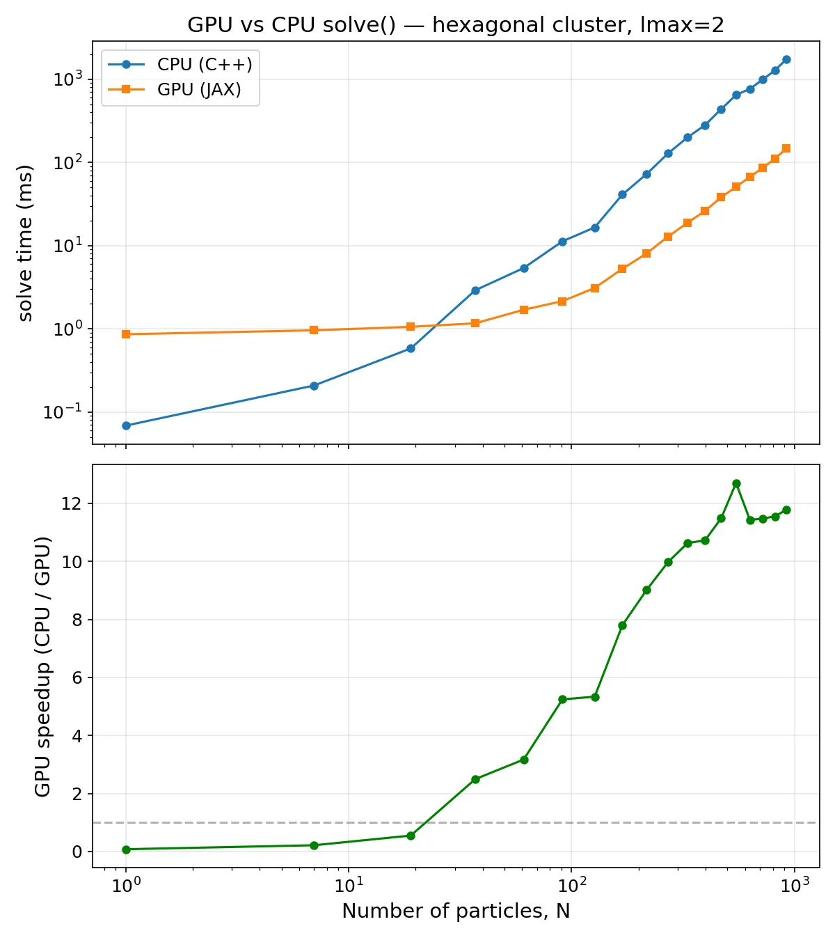
GPU vs CPU Performance
The GPU solver is in fact faster than the CPU solver for roughly . Approaching 1,000 nanoparticles, the CPU solver takes close to 6 seconds vs the GPU solver’s 0.5 seconds, a 12X speedup. This order of magnitude increase is quite significant in any scenario where the electrodynamics needs to be solved repeatedly:
- Studying optical properties at various wavelengths
- Studying different geometries and particle configurations
- Solving particle trajectories under optical tweezer illumination over longer times